SPSS Tutorials: Computing Variables: Rank Transforms (Rank Cases)

A rank variable represents the ordering of the values of a numeric variable from smallest to largest (or largest to smallest). Ranking is its own type of variable transformation, and is also useful when you want to convert a numeric variable into a categorical variable using percentiles.

In SPSS, rank transforms and percentile groupings can be computed using the Rank Cases procedure. To open Rank Cases, click Transform > Rank Cases.

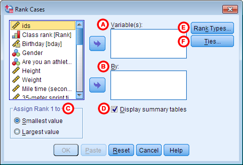
A Variables: The variables to compute rank transforms on. The new ranks will be saved to new variables (whose names will be automatically generated).

B By: (Optional) Assign ranks within groups. By variables should be nominal or ordinal, and have a small number of categories.

C Assign Rank 1 to: Should ranks be assigned in increasing or decreasing order? By default, ranks are assigned by ordering the data values in ascending order (smallest to largest), then labeling the smallest value as rank 1. Alternatively, Largest value orders the data in descending order (largest to smallest), and assigns the largest value the rank of 1.

D Display summary tables: When checked, a summary of the new rank variables is printed to the Output window. The summary includes the original variables, the name of the new variables, the rank order, the ranking method, and the method used for ties. This option is on by default.

E Rank types: (Optional) Choose one or more formulas to compute the ranks. Each box you check on this screen will add another rank variable to your dataset.

By default, only the "Rank" option is selected; this computes simple ranks. The "Ntiles" option will produce percentile-based groupings: for example, Ntiles=2 will perform a median split; Ntiles=4 will produce quartiles; Ntiles=10 will produce decile groups.

For details about the other rank types and the proportion estimation formulas, please see the official SPSS documentation for Rank Cases. Note that the Proportion Estimation Formula options are inactive unless Proportion estimates and/or Normal scores are selected.

F Ties: How should ranks be assigned in the case of ties? (A tie occurs when two or more observations share the exact same value.) There are four options for how to resolve ties: Mean, Low, High, and Sequential ranks to unique values. By default, mean ranks are assigned to ties.

• Mean - First, the observations are ordered and given unique, sequential ranks. Then, tied observations have their assigned ranks averaged together.
• Low - First, the observations are ordered and given unique, sequential ranks. Then, the ranks of any ties are re-assigned to the value of the smallest rank.
• High - First, the observations are ordered and given unique, sequential ranks. Then, the ranks of any ties are re-assigned to the value of the largest rank.
• Sequential ranks to unique values - First, the observations are ordered. Unique ranks are assigned in order until a tie is encountered. Ties receive the same rank until the next unique value appears. (The actual number of unique ranks assigned is therefore equal to the number of unique values.)

Many hypothesis tests require assumptions about the distribution of the data or residuals. A common way to adjust for non-normality is to perform a transform on that variable; for example, taking the log, square root, or square of a variable. Rank transforms are another type of transform. Suppose we want to perform a rank transform on a variable in the sample dataset that is non-normally distributed: MileMinDur.

Before the Procedure

Before we compute the ranks, let's check how many nonmissing values MileMinDur has. Let's also check the distribution of the mile run times graphically. The Frequencies procedure makes it easy to do both of these things at once:

There are two important things we want to take note of:

• The full dataset has 435 observations, but only 392 had non-missing values for their mile run time.
• The histogram shows that the mile run times are strongly skewed right; additionally, on the low end, the mile run times cut off at 5 minutes.

This means that after we run the Rank Cases procedure, the resulting variable will only have assigned ranks for the 392 cases with nonmissing mile run times.

Running the Procedure

1. Click Transform > Rank Cases.
2. Add variable MileMinDur to the Variables box.

   

3. Click Rank Types. Check the box next to Rank, then click Continue.

   

4. Click OK.

Syntax

RANK VARIABLES=MileMinDur (A)
  /RANK
  /PRINT=YES
  /TIES=MEAN.

Output

After executing the procedure, SPSS will add a new variable at the end of your dataset, and will print a table summarizing the computation in the Output window:

This table summarizes what the Rank Cases procedure did. It created a new variable named RMileMin, and assigned it the variable label "Rank of MileMinDur". It ranked the values in ascending order (i.e., the smallest value has rank 1), and it used the mean rank for values with ties.

We can inspect the new variable using the Descriptives procedure to get the sample size, minimum, maximum, mean, and standard deviation of the new variable:

Notice that we have the same sample size as the original variable (392).

For some applications, it may be more appropriate to analyze how large or small an observation is relative to others in the sample instead of looking at the raw value of the observation itself. In these instances, percentile groupings are a common way of recoding the data. Percentile groupings split the data into approximately equally sized groups, and their cutpoints will roughly correspond to the appropriate percentiles. For example, a 2-group split is equivalent to a median split; a 4-group split will split at the 25th, 50th, and 75th percentiles; and so on. The Rank Cases procedure in SPSS is capable of producing this type of grouping variable.

Before the Procedure

Let's revisit the Frequencies output from the previous example, focusing on the percentiles section:

We see that the 25th percentile is 06:39, the 50th percentile is 07:40, and the 75th percentile is 09:20. The minimum is 05:01 and the maximum is 14:02. We will keep these values in mind when we examine the results of our percentile grouping.

Running the Procedure

Using the Dialog Windows

1. Click Transform > Rank Cases.
2. Add variable MileMinDur to the Variables box.
3. Click Rank Types.
4. Check the box next to Ntiles. In the text box next to Ntiles, enter the number 4, then click Continue.
5. Click OK.

Using Syntax

RANK VARIABLES=MileMinDur (A)
  /NTILES(4)
  /PRINT=YES
  /TIES=MEAN.

Output

After executing the procedure, a new variable will be added to your active dataset. Its measurement level will automatically be set to Ordinal.

Optionally, we can check our work using the Compare Means procedure to examine the smallest and largest values that were put into each quartile group:

There are several things we can notice about how SPSS chose to handle ties and endpoints when producing these groups. In particular, recall that the 25th percentile of MileMinDur was 06:39. In this table, we see that 06:39 appears as both the maximum of group 1 and the minimum of group 2. This means that there were at least two tied observations, and the tie was resolved by putting some of the observations in the smaller group and some of the observations in the larger group.