Skip to Main Content

SPSS Tutorials: Pearson Correlation

The bivariate Pearson Correlation measures the strength and direction of linear relationships between pairs of continuous variables.

Pearson Correlation

The bivariate Pearson Correlation produces a sample correlation coefficient, r, which measures the strength and direction of linear relationships between pairs of continuous variables. By extension, the Pearson Correlation evaluates whether there is statistical evidence for a linear relationship among the same pairs of variables in the population, represented by a population correlation coefficient, ρ (“rho”). The Pearson Correlation is a parametric measure.

This measure is also known as:

  • Pearson’s correlation
  • Pearson product-moment correlation (PPMC)

Common Uses

The bivariate Pearson Correlation is commonly used to measure the following:

  • Correlations among pairs of variables
  • Correlations within and between sets of variables

The bivariate Pearson correlation indicates the following:

  • Whether a statistically significant linear relationship exists between two continuous variables
  • The strength of a linear relationship (i.e., how close the relationship is to being a perfectly straight line)
  • The direction of a linear relationship (increasing or decreasing)

Note: The bivariate Pearson Correlation cannot address non-linear relationships or relationships among categorical variables. If you wish to understand relationships that involve categorical variables and/or non-linear relationships, you will need to choose another measure of association.

Note: The bivariate Pearson Correlation only reveals associations among continuous variables. The bivariate Pearson Correlation does not provide any inferences about causation, no matter how large the correlation coefficient is.

Data Requirements

To use Pearson correlation, your data must meet the following requirements:

  1. Two or more continuous variables (i.e., interval or ratio level)
  2. Cases must have non-missing values on both variables
  3. Linear relationship between the variables
  4. Independent cases (i.e., independence of observations)
    • There is no relationship between the values of variables between cases. This means that:
      • the values for all variables across cases are unrelated
      • for any case, the value for any variable cannot influence the value of any variable for other cases
      • no case can influence another case on any variable
    • The biviariate Pearson correlation coefficient and corresponding significance test are not robust when independence is violated.
  5. Bivariate normality
    • Each pair of variables is bivariately normally distributed
    • Each pair of variables is bivariately normally distributed at all levels of the other variable(s)
    • This assumption ensures that the variables are linearly related; violations of this assumption may indicate that non-linear relationships among variables exist. Linearity can be assessed visually using a scatterplot of the data.
  6. Random sample of data from the population
  7. No outliers

Hypotheses

The null hypothesis (H0) and alternative hypothesis (H1) of the significance test for correlation can be expressed in the following ways, depending on whether a one-tailed or two-tailed test is requested:

Two-tailed significance test:

H0: ρ = 0 ("the population correlation coefficient is 0; there is no association")
H1: ρ ≠ 0 ("the population correlation coefficient is not 0; a nonzero correlation could exist")

One-tailed significance test:

H0: ρ = 0 ("the population correlation coefficient is 0; there is no association")
H1: ρ  > 0 ("the population correlation coefficient is greater than 0; a positive correlation could exist")
     OR
H1: ρ  < 0 ("the population correlation coefficient is less than 0; a negative correlation could exist")

where ρ is the population correlation coefficient.

Test Statistic

The sample correlation coefficient between two variables x and y is denoted r or rxy, and can be computed as: $$ r_{xy} = \frac{\mathrm{cov}(x,y)}{\sqrt{\mathrm{var}(x)} \dot{} \sqrt{\mathrm{var}(y)}} $$

where cov(x, y) is the sample covariance of x and y; var(x) is the sample variance of x; and var(y) is the sample variance of y.

Correlation can take on any value in the range [-1, 1]. The sign of the correlation coefficient indicates the direction of the relationship, while the magnitude of the correlation (how close it is to -1 or +1) indicates the strength of the relationship.

  •  -1 : perfectly negative linear relationship
  •   0 : no relationship
  • +1  : perfectly positive linear relationship

The strength can be assessed by these general guidelines [1] (which may vary by discipline):

  • .1 < | r | < .3 … small / weak correlation
  • .3 < | r | < .5 … medium / moderate correlation
  • .5 < | r | ……… large / strong correlation

Note: The direction and strength of a correlation are two distinct properties. The scatterplots below [2] show correlations that are r = +0.90, r = 0.00, and r = -0.90, respectively. The strength of the nonzero correlations are the same: 0.90. But the direction of the correlations is different: a negative correlation corresponds to a decreasing relationship, while and a positive correlation corresponds to an increasing relationship. 

r = -0.90

Scatterplot of data with correlation r = -0.90

r = 0.00

Scatterplot with correlation r = 0.0

r = 0.90

Scatterplot with correlation coefficient r = 0.90

Note that the r = 0.00 correlation has no discernable increasing or decreasing linear pattern in this particular graph. However, keep in mind that Pearson correlation is only capable of detecting linear associations, so it is possible to have a pair of variables with a strong nonlinear relationship and a small Pearson correlation coefficient. It is good practice to create scatterplots of your variables to corroborate your correlation coefficients.


[1]  Cohen, J. (1988). Statistical power analysis for the behavioral sciences (2nd ed.). Hillsdale, NJ: Lawrence Erlbaum Associates.

[2]  Scatterplots created in R using ggplot2, ggthemes::theme_tufte(), and MASS::mvrnorm().

Data Set-Up

Your dataset should include two or more continuous numeric variables, each defined as scale, which will be used in the analysis.

Each row in the dataset should represent one unique subject, person, or unit. All of the measurements taken on that person or unit should appear in that row. If measurements for one subject appear on multiple rows -- for example, if you have measurements from different time points on separate rows -- you should reshape your data to "wide" format before you compute the correlations.

Run a Bivariate Pearson Correlation

To run a bivariate Pearson Correlation in SPSS, click Analyze > Correlate > Bivariate.

The Bivariate Correlations window opens, where you will specify the variables to be used in the analysis. All of the variables in your dataset appear in the list on the left side. To select variables for the analysis, select the variables in the list on the left and click the blue arrow button to move them to the right, in the Variables field.

AVariables: The variables to be used in the bivariate Pearson Correlation. You must select at least two continuous variables, but may select more than two. The test will produce correlation coefficients for each pair of variables in this list.

BCorrelation Coefficients: There are multiple types of correlation coefficients. By default, Pearson is selected. Selecting Pearson will produce the test statistics for a bivariate Pearson Correlation.

CTest of Significance: Click Two-tailed or One-tailed, depending on your desired significance test. SPSS uses a two-tailed test by default.

DFlag significant correlations: Checking this option will include asterisks (**) next to statistically significant correlations in the output. By default, SPSS marks statistical significance at the alpha = 0.05 and alpha = 0.01 levels, but not at the alpha = 0.001 level (which is treated as alpha = 0.01)

EOptions: Clicking Options will open a window where you can specify which Statistics to include (i.e., Means and standard deviations, Cross-product deviations and covariances) and how to address Missing Values (i.e., Exclude cases pairwise or Exclude cases listwise). Note that the pairwise/listwise setting does not affect your computations if you are only entering two variable, but can make a very large difference if you are entering three or more variables into the correlation procedure.

Example: Understanding the linear association between weight and height

Problem Statement

Perhaps you would like to test whether there is a statistically significant linear relationship between two continuous variables, weight and height (and by extension, infer whether the association is significant in the population). You can use a bivariate Pearson Correlation to test whether there is a statistically significant linear relationship between height and weight, and to determine the strength and direction of the association.

Before the Test

In the sample data, we will use two variables: “Height” and “Weight.” The variable “Height” is a continuous measure of height in inches and exhibits a range of values from 55.00 to 84.41 (Analyze > Descriptive Statistics > Descriptives). The variable “Weight” is a continuous measure of weight in pounds and exhibits a range of values from 101.71 to 350.07.

Before we look at the Pearson correlations, we should look at the scatterplots of our variables to get an idea of what to expect. In particular, we need to determine if it's reasonable to assume that our variables have linear relationships. Click Graphs > Legacy Dialogs > Scatter/Dot. In the Scatter/Dot window, click Simple Scatter, then click Define. Move variable Height to the X Axis box, and move variable Weight to the Y Axis box. When finished, click OK.

Scatterplot of height and weight with a linear fit line added. Height and weight appear to be reasonably linearly related, albeit with some unusually outlying points.

To add a linear fit like the one depicted, double-click on the plot in the Output Viewer to open the Chart Editor. Click Elements > Fit Line at Total. In the Properties window, make sure the Fit Method is set to Linear, then click Apply. (Notice that adding the linear regression trend line will also add the R-squared value in the margin of the plot. If we take the square root of this number, it should match the value of the Pearson correlation we obtain.)

From the scatterplot, we can see that as height increases, weight also tends to increase. There does appear to be some linear relationship.

Running the Test

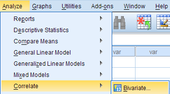
To run the bivariate Pearson Correlation, click Analyze > Correlate > Bivariate. Select the variables Height and Weight and move them to the Variables box. In the Correlation Coefficients area, select Pearson. In the Test of Significance area, select your desired significance test, two-tailed or one-tailed. We will select a two-tailed significance test in this example. Check the box next to Flag significant correlations.

Click OK to run the bivariate Pearson Correlation. Output for the analysis will display in the Output Viewer.

Syntax

CORRELATIONS
   /VARIABLES=Weight Height
   /PRINT=TWOTAIL NOSIG
   /MISSING=PAIRWISE.

Output

Tables

The results will display the correlations in a table, labeled Correlations.

Table of Pearson Correlation output. Height and weight have a significant positive correlation (r=0.513, p < 0.001).

A Correlation of Height with itself (r=1), and the number of nonmissing observations for height (n=408).

B Correlation of height and weight (r=0.513), based on n=354 observations with pairwise nonmissing values.

C Correlation of height and weight (r=0.513), based on n=354 observations with pairwise nonmissing values.

D Correlation of weight with itself (r=1), and the number of nonmissing observations for weight (n=376).

The important cells we want to look at are either B or C. (Cells B and C are identical, because they include information about the same pair of variables.) Cells B and C contain the correlation coefficient for the correlation between height and weight, its p-value, and the number of complete pairwise observations that the calculation was based on.

The correlations in the main diagonal (cells A and D) are all equal to 1. This is because a variable is always perfectly correlated with itself. Notice, however, that the sample sizes are different in cell A (n=408) versus cell D (n=376). This is because of missing data -- there are more missing observations for variable Weight than there are for variable Height.

If you have opted to flag significant correlations, SPSS will mark a 0.05 significance level with one asterisk (*) and a 0.01 significance level with two asterisks (0.01). In cell B (repeated in cell C), we can see that the Pearson correlation coefficient for height and weight is .513, which is significant (p < .001 for a two-tailed test), based on 354 complete observations (i.e., cases with nonmissing values for both height and weight).

Decision and Conclusions

Based on the results, we can state the following:

  • Weight and height have a statistically significant linear relationship (r=.513, p < .001).
  • The direction of the relationship is positive (i.e., height and weight are positively correlated), meaning that these variables tend to increase together (i.e., greater height is associated with greater weight).
  • The magnitude, or strength, of the association is approximately moderate (.3 < | r | < .5).