SPSS Tutorials: One Sample t Test

The One Sample t Test examines whether the mean of a population is statistically different from a known or hypothesized value. The One Sample t Test is a parametric test.

This test is also known as:

• Single Sample t Test

The variable used in this test is known as:

• Test variable

In a One Sample t Test, the test variable's mean is compared against a "test value", which is a known or hypothesized value of the mean in the population. Test values may come from a literature review, a trusted research organization, legal requirements, or industry standards. For example:

• A particular factory's machines are supposed to fill bottles with 150 milliliters of product. A plant manager wants to test a random sample of bottles to ensure that the machines are not under- or over-filling the bottles.
• The United States Environmental Protection Agency (EPA) sets clearance levels for the amount of lead present in homes: no more than 10 micrograms per square foot on floors and no more than 100 micrograms per square foot on window sills (as of December 2020). An inspector wants to test if samples taken from units in an apartment building exceed the clearance level.

The One Sample t Test is commonly used to test the following:

• Statistical difference between a mean and a known or hypothesized value of the mean in the population.
• Statistical difference between a change score and zero.
  • This approach involves creating a change score from two variables, and then comparing the mean change score to zero, which will indicate whether any change occurred between the two time points for the original measures. If the mean change score is not significantly different from zero, no significant change occurred.

Note: The One Sample t Test can only compare a single sample mean to a specified constant. It can not compare sample means between two or more groups. If you wish to compare the means of multiple groups to each other, you will likely want to run an Independent Samples t Test (to compare the means of two groups) or a One-Way ANOVA (to compare the means of two or more groups).

Your data must meet the following requirements:

1. Test variable that is continuous (i.e., interval or ratio level)
2. Scores on the test variable are independent (i.e., independence of observations)
   • There is no relationship between scores on the test variable
   • Violation of this assumption will yield an inaccurate p value
3. Random sample of data from the population
4. Normal distribution (approximately) of the sample and population on the test variable
   • Non-normal population distributions, especially those that are thick-tailed or heavily skewed, considerably reduce the power of the test
   • Among moderate or large samples, a violation of normality may still yield accurate p values
5. Homogeneity of variances (i.e., variances approximately equal in both the sample and population)
6. No outliers

The null hypothesis (H₀) and (two-tailed) alternative hypothesis (H₁) of the one sample T test can be expressed as:

H₀: µ =  µ₀  ("the population mean is equal to the [proposed] population mean")
H₁: µ ≠  µ₀  ("the population mean is not equal to the [proposed] population mean")

where µ is the "true" population mean and µ₀ is the proposed value of the population mean.

The test statistic for a One Sample t Test is denoted t, which is calculated using the following formula:

$$ t = \frac{\overline{x}-\mu{}_{0}}{s_{\overline{x}}} $$

where

$$ s_{\overline{x}} = \frac{s}{\sqrt{n}} $$

where

\(\mu_{0}\) = The test value -- the proposed constant for the population mean
\(\bar{x}\) = Sample mean
\(n\) = Sample size (i.e., number of observations)
\(s\) = Sample standard deviation
\(s_{\bar{x}}\) = Estimated standard error of the mean (s/sqrt(n))

The calculated t value is then compared to the critical t value from the t distribution table with degrees of freedom df = n - 1 and chosen confidence level. If the calculated t value > critical t value, then we reject the null hypothesis.

Your data should include one continuous, numeric variable (represented in a column) that will be used in the analysis. The variable's measurement level should be defined as Scale in the Variable View window.

To run a One Sample t Test in SPSS, click Analyze > Compare Means > One-Sample T Test.

The One-Sample T Test window opens where you will specify the variables to be used in the analysis. All of the variables in your dataset appear in the list on the left side. Move variables to the Test Variable(s) area by selecting them in the list and clicking the arrow button.

A Test Variable(s): The variable whose mean will be compared to the hypothesized population mean (i.e., Test Value). You may run multiple One Sample t Tests simultaneously by selecting more than one test variable. Each variable will be compared to the same Test Value. 

B Test Value: The hypothesized population mean against which your test variable(s) will be compared.

C Estimate effect sizes: Optional. If checked, will print effect size statistics -- namely, Cohen's d -- for the test(s). (Note: Effect sizes calculations for t tests were first added to SPSS Statistics in version 27, making them a relatively recent addition. If you do not see this option when you use SPSS, check what version of SPSS you're using.)

D Options: Clicking Options will open a window where you can specify the Confidence Interval Percentage and how the analysis will address Missing Values (i.e., Exclude cases analysis by analysis or Exclude cases listwise). Click Continue when you are finished making specifications.

Click OK to run the One Sample t Test.

Problem Statement

According to the CDC, the mean height of U.S. adults ages 20 and older is about 66.5 inches (69.3 inches for males, 63.8 inches for females).

In our sample data, we have a sample of 435 college students from a single college. Let's test if the mean height of students at this college is significantly different than 66.5 inches using a one-sample t test. The null and alternative hypotheses of this test will be:

H₀: µ_Height = 66.5  ("the mean height is equal to 66.5")
H₁: µ_Height ≠ 66.5  ("the mean height is not equal to 66.5")

Before the Test

In the sample data, we will use the variable Height, which a continuous variable representing each respondent’s height in inches. The heights exhibit a range of values from 55.00 to 88.41 (Analyze > Descriptive Statistics > Descriptives).

Let's create a histogram of the data to get an idea of the distribution, and to see if  our hypothesized mean is near our sample mean. Click Graphs > Legacy Dialogs > Histogram. Move variable Height to the Variable box, then click OK.

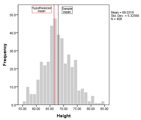
To add vertical reference lines at the mean (or another location), double-click on the plot to open the Chart Editor, then click Options > X Axis Reference Line. In the Properties window, you can enter a specific location on the x-axis for the vertical line, or you can choose to have the reference line at the mean or median of the sample data (using the sample data). Click Apply to make sure your new line is added to the chart. Here, we have added two reference lines: one at the sample mean (the solid black line), and the other at 66.5 (the dashed red line).

From the histogram, we can see that height is relatively symmetrically distributed about the mean, though there is a slightly longer right tail. The reference lines indicate that sample mean is slightly greater than the hypothesized mean, but not by a huge amount. It's possible that our test result could come back significant.

Running the Test

To run the One Sample t Test, click Analyze > Compare Means > One-Sample T Test. Move the variable Height to the Test Variable(s) area. In the Test Value field, enter 66.5.

Click OK to run the One Sample t Test.

Syntax

If you are using SPSS Statistics 27 or later:

T-TEST
  /TESTVAL=66.5
  /MISSING=ANALYSIS
  /VARIABLES=Height
  /ES DISPLAY(TRUE)
  /CRITERIA=CI(.95).

If you are using SPSS Statistics 26 or earlier:

T-TEST
   /TESTVAL=66.5
   /MISSING=ANALYSIS
   /VARIABLES=Height
   /CRITERIA=CI(.95).

Output

Tables

Two sections (boxes) appear in the output: One-Sample Statistics and One-Sample Test. The first section, One-Sample Statistics, provides basic information about the selected variable, Height, including the valid (nonmissing) sample size (n), mean, standard deviation, and standard error. In this example, the mean height of the sample is 68.03 inches, which is based on 408 nonmissing observations.

The second section, One-Sample Test, displays the results most relevant to the One Sample t Test. 

A Test Value: The number we entered as the test value in the One-Sample T Test window.

B t Statistic: The test statistic of the one-sample t test, denoted t. In this example, t = 5.810. Note that t is calculated by dividing the mean difference (E) by the standard error mean (from the One-Sample Statistics box).

C df: The degrees of freedom for the test. For a one-sample t test, df = n - 1; so here, df = 408 - 1 = 407.

D Significance (One-Sided p and Two-Sided p): The p-values corresponding to one of the possible one-sided alternative hypotheses (in this case, µ_Height > 66.5) and two-sided alternative hypothesis (µ_Height ≠ 66.5), respectively. In our problem statement above, we were only interested in the two-sided alternative hypothesis.

E Mean Difference: The difference between the "observed" sample mean (from the One Sample Statistics box) and the "expected" mean (the specified test value (A)). The sign of the mean difference corresponds to the sign of the t value (B). The positive t value in this example indicates that the mean height of the sample is greater than the hypothesized value (66.5).

F Confidence Interval for the Difference: The confidence interval for the difference between the specified test value and the sample mean.

Decision and Conclusions

Recall that our hypothesized population value was 66.5 inches, the [approximate] average height of the overall adult population in the U.S. Since p < 0.001, we reject the null hypothesis that the mean height of students at this college is equal to the hypothesized population mean of 66.5 inches and conclude that the mean height is significantly different than 66.5 inches.

Based on the results, we can state the following:

• There is a significant difference in the mean height of the students at this college and the overall adult population in the U.S. (p < .001).
• The average height of students at this college is about 1.5 inches taller than the U.S. adult population average (95% CI [1.013, 2.050]).