Problem Statement
In our sample dataset, students reported their typical time to run a mile, and whether or not they were an athlete. Suppose we want to know if the average time to run a mile is different for athletes versus non-athletes. This involves testing whether the sample means for mile time among athletes and non-athletes in your sample are statistically different (and by extension, inferring whether the means for mile times in the population are significantly different between these two groups). You can use an Independent Samples t Test to compare the mean mile time for athletes and non-athletes.
The hypotheses for this example can be expressed as:
H0: µnon-athlete − µathlete = 0 ("the difference of the means is equal to zero")
H1: µnon-athlete − µathlete ≠ 0 ("the difference of the means is not equal to zero")
where µathlete and µnon-athlete are the population means for athletes and non-athletes, respectively.
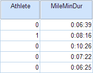
In the sample data, we will use two variables: Athlete and MileMinDur. The variable Athlete has values of either “0” (non-athlete) or "1" (athlete). It will function as the independent variable in this T test. The variable MileMinDur is a numeric duration variable (h:mm:ss), and it will function as the dependent variable. In SPSS, the first few rows of data look like this:
Before the Test
Before running the Independent Samples t Test, it is a good idea to look at descriptive statistics and graphs to get an idea of what to expect. Running Compare Means (Analyze > Compare Means and Proportions > Means) to get descriptive statistics by group tells us that the standard deviation in mile time for non-athletes is about 2 minutes; for athletes, it is about 49 seconds. This corresponds to a variance of 14803 seconds for non-athletes, and a variance of 2447 seconds for athletes1. Running the Explore procedure (Analyze > Descriptives > Explore) to obtain a comparative boxplot yields the following graph:

If the variances were indeed equal, we would expect the total length of the boxplots to be about the same for both groups. However, from this boxplot, it is clear that the spread of observations for non-athletes is much greater than the spread of observations for athletes. Already, we can estimate that the variances for these two groups are quite different. It should not come as a surprise if we run the Independent Samples t Test and see that Levene's Test is significant.
Additionally, we should also decide on a significance level (typically denoted using the Greek letter alpha, α) before we perform our hypothesis tests. The significance level is the threshold we use to decide whether a test result is significant. For this example, let's use α = 0.05.
1When computing the variance of a duration variable (formatted as hh:mm:ss or mm:ss or mm:ss.s), SPSS converts the standard deviation value to seconds before squaring.
Running the Test
To run the Independent Samples t Test:
- Click Analyze > Compare Means and Proportions > Independent-Samples T Test.
- Move the variable Athlete to the Grouping Variable field, and move the variable MileMinDur to the Test Variable(s) area. Now Athlete is defined as the independent variable and MileMinDur is defined as the dependent variable.
- Click Define Groups, which opens a new window. Use specified values is selected by default. Since our grouping variable is numerically coded (0 = "Non-athlete", 1 = "Athlete"), type “0” in the first text box, and “1” in the second text box. This indicates that we will compare groups 0 and 1, which correspond to non-athletes and athletes, respectively. Click Continue when finished.
- If you are using SPSS Statistics version 27 or later: Click the box next to Estimate effect sizes so that it is selected.
- If you are using SPSS Statistics version 31 or later: Click the box next to Homogeneity of variance test so that it is selected.
- Click OK to run the Independent Samples t Test. Output for the analysis will display in the Output Viewer window.
Syntax
Most SPSS Versions
T-TEST GROUPS=Athlete(0 1)
   /MISSING=ANALYSIS
   /VARIABLES=MileMinDur
   /CRITERIA=CI(.95).
SPSS Versions 27 and Later
T-TEST GROUPS=Athlete(0 1)
  /MISSING=ANALYSIS
  /VARIABLES=MileMinDur
  /ES DISPLAY(TRUE)
  /CRITERIA=CI(.95).
SPSS Versions 31 and Later
T-TEST GROUPS=Athlete(0 1)
  /MISSING=ANALYSIS
  /VARIABLES=MileMinDur
  /ES DISPLAY(TRUE)
  /HOMOGENEITY DISPLAY(TRUE)
  /CRITERIA=CI(.95).
Output
Tables
Assuming that you enabled the Effect Size and Homogeneity of Variance Test options, the output will have four sections (boxes): Group Statistics, Independent Samples Test, Homogeneity of Variance Test, and Independent Samples Effect Sizes.
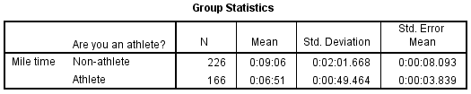
Group Statistics
The first section, Group Statistics, provides basic information about the group comparisons, including the sample size (n), mean, standard deviation, and standard error for mile times by group. In this example, there are 166 athletes and 226 non-athletes. The mean mile time for athletes is 6 minutes 51 seconds, and the mean mile time for non-athletes is 9 minutes 6 seconds.
Independent Samples Test
The second section, Independent Samples Test, displays the results most relevant to the Independent Samples t Test. Depending on your version of SPSS Statistics, you may see Levene's Test results in this table.

From left to right:
- t is the computed test statistic, using the formula for the equal-variances-assumed test statistic (first row of table) or the formula for the equal-variances-not-assumed test statistic (second row of table)
- df is the degrees of freedom, using the equal-variances-assumed degrees of freedom formula (first row of table) or the equal-variances-not-assumed degrees of freedom formula (second row of table)
- Significance contains the one-sided and two-sided p-values corresponding to the given test statistic and degrees of freedom
- Mean Difference is the difference between the sample means, i.e. x1 − x2; it also corresponds to the numerator of the test statistic for that test
- Std. Error Difference is the standard error of the mean difference estimate; it also corresponds to the denominator of the test statistic for that test
- Confidence Interval of the Difference: This part of the t-test output complements the significance test results. Typically, if the CI for the mean difference contains 0 within the interval -- i.e., if the lower boundary of the CI is a negative number and the upper boundary of the CI is a positive number -- the results are not significant at the chosen significance level
Note that the mean difference is calculated by subtracting the mean of the second group from the mean of the first group. In this example, the mean mile time for athletes was subtracted from the mean mile time for non-athletes (9:06 minus 6:51 = 02:14). The sign of the mean difference corresponds to the sign of the t value. The positive t value in this example indicates that the mean mile time of the first group, non-athletes, is greater than the mean mile time of the second group, athletes.
Which row of the table should we look at? It depends on whether we believe the variance of the dependent variable is the same for both groups. Based on Levene's test (below), we would focus on the "Equal variances not assumed" row. In that case, the two-sided p-value is less than .001, which is below our chosen significance level α = .05, so we reject the null and conclude in favor of the alternative hypothesis: that the mean mile run time of the athletes is significantly different than the mean mile run time of the non-athletes.
Homogeneity of Variance Test
The third section, Homogeneity of Variance test, contains the Levene's Test results.

From left to right:
- F is the test statistic of Levene's test
- Sig. is the p-value corresponding to this test statistic.
The p-value of Levene's test is printed as p < 0.001 -- i.e., p very small -- so we we reject the null of Levene's test and conclude that the variance in mile time of athletes is significantly different than that of non-athletes. This suggests that we should look at the "Equal variances not assumed" row for the t test (and corresponding confidence interval) results. (If this test result had not been significant -- that is, if we had observed p > .05 -- then we would have used the "Equal variances assumed" output.)
Independent Samples Effect Sizes
The fourth section, Independent Samples Effect Sizes, contains the calculated effect sizes.

The primary column of interest in this table is the Point Estimate column.
Effect sizes are measures of the magnitude of the difference between groups or the strength of association between groups. While p-values tell us whether a statistically significant difference between groups exists (i.e., observed differences are not likely due to chance), effect sizes tell us how small or large that difference is by estimating how many standard deviation units the group means are from each other. Effect sizes are useful as they give us a more practical understanding of the significant difference or association between groups.
As the Independent Samples Effect Sizes table shows, there are three effect size measures for independent samples t tests: Cohen’s d, Hedges’ correction (also known as Hedges’ g), and Glass’s delta.
Cohen’s d and Hedges’ Correction
Both formulas are used to measure the standardized (i.e., standard deviation units) separation of two groups. A measure of 1.0 indicates that the group means are separated by one standard deviation, 2.0 means a separation of two standard deviations, etc. Effect sizes range from:
0.20 = small effect
0.50 = medium effect
0.80+ = large effect
Cohen’s d is calculated by subtracting the mean of group 2 (athletes) from the mean of group 1 (non-athletes) and dividing the difference by the pooled standard deviation. For our mile run time example, the first number in the Point Estimate column is Cohen’s d, which is 1.377. This means that the mean mile run time of non-athletes is separated from the mean mile run time of athletes by 1.377 standard deviations. Referring to the threshold chart above, this means there is a large effect.
Hedges’ correction is calculated by multiplying Cohen’s d by a correction factor. This correction factor was created to calculate a more conservative estimate of effect size, particularly in the case of small sample sizes. Generally, Hedges’ correction will be very close to Cohen’s d, as seen in the Point Estimate column in the table above. Hedges’ correction is 1.375, meaning that the mean mile run time of non-athletes is separated from the mean mile run time of athletes by 1.375 standard deviations. This is a large effect size.
Glass’s delta
Also measures the magnitude of separation between two groups, primarily when one group is a control group and the other is a treatment group. In SPSS, what we identify as Group 1 (in this example, “Non-athlete”) is the treatment group and Group 2 (“Athlete”) is the control group. Glass’s delta is calculated by subtracting the control group mean from the treatment group mean and dividing the difference by the standard deviation of the control group. This tends to produce a different estimate than Cohen’s d and Hedges’ correction—the standard deviation of a control group will usually be different than a pooled standard deviation, meaning Glass’s delta uses a different denominator than Cohen’s d and Hedges’ correction. Directionality also matters when interpreting Glass’s delta; a negative value means the treatment group’s mean is higher than the control, while a positive value means the treatment group’s mean is lower than the control. However, a positive or negative value does not influence the size of the effect, as effect sizes are interpreted based on the absolute value.
The Point Estimate column shows us that Glass’s delta is 2.725, meaning that the mean mile run time of non-athletes is higher than the mean mile run time of athletes and the means are separated by 2.725 standard deviation units. But we must ask ourselves if, given our example, it makes sense to interpret Glass’s delta? Recall that our hypothesis stated that the means of the two groups are not equal, but we did not specify that one group was a control and that the other would be exposed to a treatment that would be expected to produce a different mean. Therefore, our hypothetical research design does not justify the interpretation of Glass’s delta.
Decision and Conclusions
Since p < .001 is less than our chosen significance level α = 0.05, we can reject the null hypothesis, and conclude that the that the mean mile time for athletes and non-athletes is significantly different.
Based on the results, we can state the following:
- There was a significant difference in mean mile time between non-athletes and athletes (t315.846 = 15.047, p < .001).
- The average mile time for athletes was 2 minutes and 14 seconds lower than the average mile time for non-athletes.
- Cohen's d indicates that the group means are separated by 1.377 standard deviations, meaning there is a large effect.


