Skip to Main Content

SPSS Tutorials: Chi-Square Test of Independence

The Chi-Square Test of Independence is used to test if two categorical variables are associated.

Chi-Square Test of Independence

The Chi-Square Test of Independence determines whether there is an association between categorical variables (i.e., whether the variables are independent or related). It is a nonparametric test.

This test is also known as:

  • Chi-Square Test of Association.

This test utilizes a contingency table to analyze the data. A contingency table (also known as a cross-tabulation, crosstab, or two-way table) is an arrangement in which data is classified according to two categorical variables. The categories for one variable appear in the rows, and the categories for the other variable appear in columns. Each variable must have two or more categories. Each cell reflects the total count of cases for a specific pair of categories.

There are several tests that go by the name "chi-square test" in addition to the Chi-Square Test of Independence. Look for context clues in the data and research question to make sure what form of the chi-square test is being used.

Common Uses

The Chi-Square Test of Independence is commonly used to test the following:

  • Statistical independence or association between two categorical variables.

The Chi-Square Test of Independence can only compare categorical variables. It cannot make comparisons between continuous variables or between categorical and continuous variables. Additionally, the Chi-Square Test of Independence only assesses associations between categorical variables, and can not provide any inferences about causation.

If your categorical variables represent "pre-test" and "post-test" observations, then the chi-square test of independence is not appropriate. This is because the assumption of the independence of observations is violated. In this situation, McNemar's Test is appropriate.

Data Requirements

Your data must meet the following requirements:

  1. Two categorical variables.
  2. Two or more categories (groups) for each variable.
  3. Independence of observations.
    • There is no relationship between the subjects in each group.
    • The categorical variables are not "paired" in any way (e.g. pre-test/post-test observations).
  4. Relatively large sample size.
    • Expected frequencies for each cell are at least 1.
    • Expected frequencies should be at least 5 for the majority (80%) of the cells.

Hypotheses

The null hypothesis (H0) and alternative hypothesis (H1) of the Chi-Square Test of Independence can be expressed in two different but equivalent ways:

H0: "[Variable 1] is independent of [Variable 2]"
H1: "[Variable 1] is not independent of [Variable 2]"

OR

H0: "[Variable 1] is not associated with [Variable 2]"
H1"[Variable 1] is associated with [Variable 2]"

Test Statistic

The test statistic for the Chi-Square Test of Independence is denoted Χ2, and is computed as:

$$ \chi^{2} = \sum_{i=1}^{R}{\sum_{j=1}^{C}{\frac{(o_{ij} - e_{ij})^{2}}{e_{ij}}}} $$

where

\(o_{ij}\) is the observed cell count in the ith row and jth column of the table

\(e_{ij}\) is the expected cell count in the ith row and jth column of the table, computed as

$$ e_{ij} = \frac{\mathrm{ \textrm{row } \mathit{i}} \textrm{ total} * \mathrm{\textrm{col } \mathit{j}} \textrm{ total}}{\textrm{grand total}} $$

The quantity (oij - eij) is sometimes referred to as the residual of cell (i, j), denoted \(r_{ij}\).

The calculated Χ2 value is then compared to the critical value from the Χ2 distribution table with degrees of freedom df = (R - 1)(C - 1) and chosen confidence level. If the calculated Χ2 value > critical Χ2 value, then we reject the null hypothesis.

Data Set-Up

There are two different ways in which your data may be set up initially. The format of the data will determine how to proceed with running the Chi-Square Test of Independence. At minimum, your data should include two categorical variables (represented in columns) that will be used in the analysis. The categorical variables must include at least two groups. Your data may be formatted in either of the following ways:

If you have the raw data (each row is a subject):

Example of a dataset structure where each row represents a case or subject. Screenshot shows a Data View window with cases 1-5 and 430-435 from the sample dataset, and columns ids, Smoking and Gender.

  • Cases represent subjects, and each subject appears once in the dataset. That is, each row represents an observation from a unique subject.
  • The dataset contains at least two nominal categorical variables (string or numeric). The categorical variables used in the test must have two or more categories.

If you have frequencies (each row is a combination of factors):

An example of using the chi-square test for this type of data can be found in the Weighting Cases tutorial.

Example of a dataset structure where each row represents a frequency. Screenshot shows a Data View window with three columns (ClassRank, PickedAMajor, and Freq) and six rows.

  • Cases represent the combinations of categories for the variables.
    • Each row in the dataset represents a distinct combination of the categories.
    • The value in the "frequency" column for a given row is the number of unique subjects with that combination of categories.
  • You should have three variables: one representing each category, and a third representing the number of occurrences of that particular combination of factors.
  • Before running the test, you must activate Weight Cases, and set the frequency variable as the weight.

Run a Chi-Square Test of Independence

In SPSS, the Chi-Square Test of Independence is an option within the Crosstabs procedure. Recall that the Crosstabs procedure creates a contingency table or two-way table, which summarizes the distribution of two categorical variables.

To create a crosstab and perform a chi-square test of independence, click Analyze > Descriptive Statistics > Crosstabs.

A Row(s): One or more variables to use in the rows of the crosstab(s). You must enter at least one Row variable.

B Column(s): One or more variables to use in the columns of the crosstab(s). You must enter at least one Column variable.

Also note that if you specify one row variable and two or more column variables, SPSS will print crosstabs for each pairing of the row variable with the column variables. The same is true if you have one column variable and two or more row variables, or if you have multiple row and column variables. A chi-square test will be produced for each table. Additionally, if you include a layer variable, chi-square tests will be run for each pair of row and column variables within each level of the layer variable.

C Layer: An optional "stratification" variable. If you have turned on the chi-square test results and have specified a layer variable, SPSS will subset the data with respect to the categories of the layer variable, then run chi-square tests between the row and column variables. (This is not equivalent to testing for a three-way association, or testing for an association between the row and column variable after controlling for the layer variable.)


D Statistics: Opens the Crosstabs: Statistics window, which contains fifteen different inferential statistics for comparing categorical variables.

In the Crosstabs: Statistics window, check the box next to Chi-square.

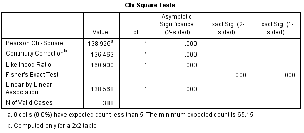
To run the Chi-Square Test of Independence, make sure that the Chi-square box is checked.


E Cells: Opens the Crosstabs: Cell Display window, which controls which output is displayed in each cell of the crosstab. (Note: in a crosstab, the cells are the inner sections of the table. They show the number of observations for a given combination of the row and column categories.) There are three options in this window that are useful (but optional) when performing a Chi-Square Test of Independence:

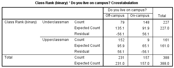
1Observed: The actual number of observations for a given cell. This option is enabled by default.

2Expected: The expected number of observations for that cell (see the test statistic formula).

3Unstandardized Residuals: The "residual" value, computed as observed minus expected.


F Format: Opens the Crosstabs: Table Format window, which specifies how the rows of the table are sorted.

Example: Chi-square Test for 3x2 Table

Problem Statement

In the sample dataset, respondents were asked their gender and whether or not they were a cigarette smoker. There were three answer choices: Nonsmoker, Past smoker, and Current smoker. Suppose we want to test for an association between smoking behavior (nonsmoker, current smoker, or past smoker) and gender (male or female) using a Chi-Square Test of Independence (we'll use α = 0.05).

Before the Test

Before we test for "association", it is helpful to understand what an "association" and a "lack of association" between two categorical variables looks like. One way to visualize this is using clustered bar charts. Let's look at the clustered bar chart produced by the Crosstabs procedure.

This is the chart that is produced if you use Smoking as the row variable and Gender as the column variable (running the syntax later in this example):

The "clusters" in a clustered bar chart are determined by the row variable (in this case, the smoking categories). The color of the bars is determined by the column variable (in this case, gender). The height of each bar represents the total number of observations in that particular combination of categories.

This type of chart emphasizes the differences within the categories of the row variable. Notice how within each smoking category, the heights of the bars (i.e., the number of males and females) are very similar. That is, there are an approximately equal number of male and female nonsmokers; approximately equal number of male and female past smokers; approximately equal number of male and female current smokers. If there were an association between gender and smoking, we would expect these counts to differ between groups in some way.

Running the Test

  1. Open the Crosstabs dialog (Analyze > Descriptive Statistics > Crosstabs).
  2. Select Smoking as the row variable, and Gender as the column variable.
  3. Click Statistics. Check Chi-square, then click Continue.
  4. (Optional) Check the box for Display clustered bar charts.
  5. Click OK.

Syntax

CROSSTABS
  /TABLES=Smoking BY Gender
  /FORMAT=AVALUE TABLES
  /STATISTICS=CHISQ
  /CELLS=COUNT
  /COUNT ROUND CELL
  /BARCHART.

Output

Tables

The first table is the Case Processing summary, which tells us the number of valid cases used for analysis. Only cases with nonmissing values for both smoking behavior and gender can be used in the test.

Case Processing Summary table for the crosstab of smoking by gender. There are 402 valid cases (92.4%) and 33 cases with missing values on one or both variables (7.6%).

The next tables are the crosstabulation and chi-square test results.

Crosstabulation between smoking and gender, based on 402 valid cases.

Chi-square test based on the crosstab of smoking and gender. The Pearson Chi-square statistic is 3.171 with 2 degrees of freedom and a 2-sided p-value of 0.205.

The key result in the Chi-Square Tests table is the Pearson Chi-Square.

  • The value of the test statistic is 3.171.
  • The footnote for this statistic pertains to the expected cell count assumption (i.e., expected cell counts are all greater than 5): no cells had an expected count less than 5, so this assumption was met.
  • Because the test statistic is based on a 3x2 crosstabulation table, the degrees of freedom (df) for the test statistic is $$ df = (R - 1)*(C - 1) = (3 - 1)*(2 - 1) = 2*1 = 2 $$.
  • The corresponding p-value of the test statistic is p = 0.205.

Decision and Conclusions

Since the p-value is greater than our chosen significance level (α = 0.05), we do not reject the null hypothesis. Rather, we conclude that there is not enough evidence to suggest an association between gender and smoking.

Based on the results, we can state the following:

  • No association was found between gender and smoking behavior (Χ2(2)> = 3.171, p = 0.205).

Example: Chi-square Test for 2x2 Table

Problem Statement

Let's continue the row and column percentage example from the Crosstabs tutorial, which described the relationship between the variables RankUpperUnder (upperclassman/underclassman) and LivesOnCampus (lives on campus/lives off-campus). Recall that the column percentages of the crosstab appeared to indicate that upperclassmen were less likely than underclassmen to live on campus:

  • The proportion of underclassmen who live off campus is 34.8%, or 79/227.
  • The proportion of underclassmen who live on campus is 65.2%, or 148/227.
  • The proportion of upperclassmen who live off campus is 94.4%, or 152/161.
  • The proportion of upperclassmen who live on campus is 5.6%, or 9/161.

Suppose that we want to test the association between class rank and living on campus using a Chi-Square Test of Independence (using α = 0.05).

Before the Test

The clustered bar chart from the Crosstabs procedure can act as a complement to the column percentages above. Let's look at the chart produced by the Crosstabs procedure for this example:

The height of each bar represents the total number of observations in that particular combination of categories. The "clusters" are formed by the row variable (in this case, class rank). This type of chart emphasizes the differences within the underclassmen and upperclassmen groups. Here, the differences in number of students living on campus versus living off-campus is much starker within the class rank groups.

Running the Test

  1. Open the Crosstabs dialog (Analyze > Descriptive Statistics > Crosstabs).
  2. Select RankUpperUnder as the row variable, and LiveOnCampus as the column variable.
  3. Click Statistics. Check Chi-square, then click Continue.
  4. (Optional) Click Cells. Under Counts, check the boxes for Observed and Expected, and under Residuals, click Unstandardized. Then click Continue.
  5. (Optional) Check the box for Display clustered bar charts.
  6. Click OK.

Output

Syntax

CROSSTABS
  /TABLES=RankUpperUnder BY LiveOnCampus
  /FORMAT=AVALUE TABLES
  /STATISTICS=CHISQ 
  /CELLS=COUNT EXPECTED RESID 
  /COUNT ROUND CELL
  /BARCHART.

Tables

The first table is the Case Processing summary, which tells us the number of valid cases used for analysis. Only cases with nonmissing values for both class rank and living on campus can be used in the test.

The case processing summary for the crosstab of class rank by living on campus. There were 388 valid cases (89.2%) and 47 cases with missing values of one or both variables (10.8%).

The next table is the crosstabulation. If you elected to check off the boxes for Observed Count, Expected Count, and Unstandardized Residuals, you should see the following table:

The crosstabulation of class rank by living on campus.

With the Expected Count values shown, we can confirm that all cells have an expected value greater than 5.

Computation of the expected cell counts and residuals (observed minus expected) for the crosstabulation of class rank by living on campus.
  Off-Campus On-Campus Total
Underclassman

Row 1, column 1

$$ o_{\mathrm{11}} = 79 $$

$$ e_{\mathrm{11}} = \frac{227*231}{388} = 135.147 $$

$$ r_{\mathrm{11}} = 79 - 135.147 = -56.147 $$

Row 1, column 2

$$ o_{\mathrm{12}} = 148 $$

$$ e_{\mathrm{12}} = \frac{227*157}{388} = 91.853 $$

$$ r_{\mathrm{12}} = 148 - 91.853 = 56.147 $$

row 1 total = 227
Upperclassmen

Row 2, column 1

$$ o_{\mathrm{21}} = 152 $$

$$ e_{\mathrm{21}} = \frac{161*231}{388} = 95.853 $$

$$ r_{\mathrm{21}} = 152 - 95.853 = 56.147 $$

Row 2, column 2

$$ o_{\mathrm{22}} = 9 $$

$$ e_{\mathrm{22}} = \frac{161*157}{388} = 65.147 $$

$$ r_{\mathrm{22}} = 9 - 65.147 = -56.147 $$

row 2 total = 161
Total col 1 total = 231 col 2 total = 157 grand total = 388

These numbers can be plugged into the chi-square test statistic formula:

$$ \chi^{2} = \sum_{i=1}^{R}{\sum_{j=1}^{C}{\frac{(o_{ij} - e_{ij})^{2}}{e_{ij}}}} = \frac{(-56.147)^{2}}{135.147} + \frac{(56.147)^{2}}{91.853} + \frac{(56.147)^{2}}{95.853} + \frac{(-56.147)^{2}}{65.147} = 138.926 $$

We can confirm this computation with the results in the Chi-Square Tests table:

The table of chi-square test results, based on the crosstab of class rank by living on campus. The Pearson chi-square test statistic is 138.926 with 1 degree of freedom and a p-value less than 0.001.

The row of interest here is Pearson Chi-Square and its footnote.

  • The value of the test statistic is 138.926.
  • The footnote for this statistic pertains to the expected cell count assumption (i.e., expected cell counts are all greater than 5): no cells had an expected count less than 5, so this assumption was met.
  • Because the crosstabulation is a 2x2 table, the degrees of freedom (df) for the test statistic is $$ df = (R - 1)*(C - 1) = (2 - 1)*(2 - 1) = 1 $$.
  • The corresponding p-value of the test statistic is so small that it is cut off from display. Instead of writing "p = 0.000", we instead write the mathematically correct statement p < 0.001.

Decision and Conclusions

Since the p-value is less than our chosen significance level α = 0.05, we can reject the null hypothesis, and conclude that there is an association between class rank and whether or not students live on-campus.

Based on the results, we can state the following:

  • There was a significant association between class rank and living on campus (Χ2(1) = 138.9, p < .001).