SAS Tutorials: Pearson Correlation with PROC CORR

The bivariate Pearson Correlation produces a sample correlation coefficient, r, which measures the strength and direction of linear relationships between pairs of continuous variables. By extension, the Pearson Correlation evaluates whether there is statistical evidence for a linear relationship among the same pairs of variables in the population, represented by a population correlation coefficient, ρ (“rho”). The Pearson Correlation is a parametric measure.

This measure is also known as:

• Pearson’s correlation
• Pearson product-moment correlation (PPMC)

The bivariate Pearson Correlation is commonly used to measure the following:

• Correlations among pairs of variables
• Correlations within and between sets of variables

The bivariate Pearson correlation indicates the following:

• Whether a statistically significant linear relationship exists between two continuous variables
• The strength of a linear relationship (i.e., how close the relationship is to being a perfectly straight line)
• The direction of a linear relationship (increasing or decreasing)

Note: The bivariate Pearson Correlation cannot address non-linear relationships or relationships among categorical variables. If you wish to understand relationships that involve categorical variables and/or non-linear relationships, you will need to choose another measure of association.

Note: The bivariate Pearson Correlation only reveals associations among continuous variables. The bivariate Pearson Correlation does not provide any inferences about causation, no matter how large the correlation coefficient is.

To use Pearson correlation, your data must meet the following requirements:

1. Two or more continuous variables (i.e., interval or ratio level)
2. Cases must have non-missing values on both variables
3. Linear relationship between the variables
4. Independent cases (i.e., independence of observations)
   • There is no relationship between the values of variables between cases. This means that:
     • the values for all variables across cases are unrelated
     • for any case, the value for any variable cannot influence the value of any variable for other cases
     • no case can influence another case on any variable
   • The biviariate Pearson correlation coefficient and corresponding significance test are not robust when independence is violated.
5. Bivariate normality
   • Each pair of variables is bivariately normally distributed
   • Each pair of variables is bivariately normally distributed at all levels of the other variable(s)
   • This assumption ensures that the variables are linearly related; violations of this assumption may indicate that non-linear relationships among variables exist. Linearity can be assessed visually using a scatterplot of the data.
6. Random sample of data from the population
7. No outliers

The null hypothesis (H₀) and alternative hypothesis (H₁) of the significance test for correlation can be expressed in the following ways, depending on whether a one-tailed or two-tailed test is requested:

Two-tailed significance test:

H₀: ρ = 0 ("the population correlation coefficient is 0; there is no association")
H₁: ρ ≠ 0 ("the population correlation coefficient is not 0; a nonzero correlation could exist")

One-tailed significance test:

H₀: ρ = 0 ("the population correlation coefficient is 0; there is no association")
H₁: ρ  > 0 ("the population correlation coefficient is greater than 0; a positive correlation could exist")
     OR
H₁: ρ  < 0 ("the population correlation coefficient is less than 0; a negative correlation could exist")

where ρ is the population correlation coefficient.

The sample correlation coefficient between two variables x and y is denoted r or r_xy, and can be computed as: $$ r_{xy} = \frac{\mathrm{cov}(x,y)}{\sqrt{\mathrm{var}(x)} \dot{} \sqrt{\mathrm{var}(y)}} $$

where cov(x, y) is the sample covariance of x and y; var(x) is the sample variance of x; and var(y) is the sample variance of y.

Correlation can take on any value in the range [-1, 1]. The sign of the correlation coefficient indicates the direction of the relationship, while the magnitude of the correlation (how close it is to -1 or +1) indicates the strength of the relationship.

•  -1 : perfectly negative linear relationship
•   0 : no relationship
• +1  : perfectly positive linear relationship

The strength can be assessed by these general guidelines [1] (which may vary by discipline):

• .1 < | r | < .3 … small / weak correlation
• .3 < | r | < .5 … medium / moderate correlation
• .5 < | r | ……… large / strong correlation

Note: The direction and strength of a correlation are two distinct properties. The scatterplots below [2] show correlations that are r = +0.90, r = 0.00, and r = -0.90, respectively. The strength of the nonzero correlations are the same: 0.90. But the direction of the correlations is different: a negative correlation corresponds to a decreasing relationship, while and a positive correlation corresponds to an increasing relationship. 

Note that the r = 0.00 correlation has no discernable increasing or decreasing linear pattern in this particular graph. However, keep in mind that Pearson correlation is only capable of detecting linear associations, so it is possible to have a pair of variables with a strong nonlinear relationship and a small Pearson correlation coefficient. It is good practice to create scatterplots of your variables to corroborate your correlation coefficients.

[1]  Cohen, J. (1988). Statistical power analysis for the behavioral sciences (2nd ed.). Hillsdale, NJ: Lawrence Erlbaum Associates.

[2]  Scatterplots created in R using ggplot2, ggthemes::theme_tufte(), and MASS::mvrnorm().

Your data should include two or more continuous numeric variables.

The CORR procedure produces Pearson correlation coefficients of continuous numeric variables. The basic syntax of the CORR procedure is: 

PROC CORR DATA=dataset <options>;
    VAR variable(s);
    WITH variable(s);
RUN;

In the first line of the SAS code above, PROC CORR tells SAS to execute the CORR procedure on the dataset given in the DATA= argument. Immediately following PROC CORR is where you put any procedure-level options you want to include. Let’s review some of the more common options:

• NOMISS
  Excludes observations with missing values on any of the analysis variables specified in the VAR or WITH statements (i.e., listwise exclusion).
• PLOTS=MATRIX
  Creates a scatterplot matrix of the variables in the VAR and/or WITH statements.
• PLOTS=MATRIX(HISTOGRAM)
  Same as above, but changes the panels on the diagonal of the scatterplot matrix to display histograms of the variables in the VAR statement. (The HISTOGRAM option is ignored if you include a WITH statement.)
• PLOTS=SCATTER
  Creates individual scatterplots of the variables in the VAR and/or WITH statements.
• PLOTS(MAXPOINTS=n)=<...>
  Used to increase the limit on the number of datapoints used in a plot to some number n. By default, n is 5000. Can be used in conjunction with any of the above options for MATRIX and SCATTER. If you have included PLOTS syntax in your script but do not see any plots in your output, check your log window; if you see the message

  WARNING: The scatter plot matrix with more than 5000 points has been suppressed. Use the
           PLOTS(MAXPOINTS= ) option in the PROC CORR statement to change or override the cutoff.

  then you should try revising the code to PLOTS(MAXPOINTS=15000)= and rerun.

On the next line, the VAR statement is where you specify all of the variables you want to compute pairwise correlations for. You can list as many variables as you want, with each variable separated by a space. If the VAR statement is not included, then SAS will include every numeric variable that does not appear in any other of the statements.

The WITH statement is optional, but is typically used if you only want to run correlations between certain combinations of variables. If both the VAR and WITH statements are used, each variable in the WITH statement will be correlated against each variable in the VAR statement.

When ODS graphics are turned on and you request plots from PROC CORR, each plot will be saved as a PNG file in the same directory where your SAS code is. If you run the same code multiple times, it will create new graphics files for each run (rather than overwriting the old ones).

Problem Statement

Perhaps you would like to test whether there is a statistically significant linear relationship between two continuous variables, weight and height (and by extension, infer whether the association is significant in the population). You can use a bivariate Pearson Correlation to test whether there is a statistically significant linear relationship between height and weight, and to determine the strength and direction of the association.

Before the Test

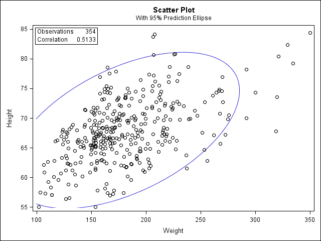
Before we look at the Pearson correlations, we should look at the scatterplots of our variables to get an idea of what to expect. In particular, we need to determine if it's reasonable to assume that our variables have linear relationships. PROC CORR automatically includes descriptive statistics (including mean, standard deviation, minimum, and maximum) for the input variables, and can optionally create scatterplots and/or scatterplot matrices. (Note that the plots require the ODS graphics system. If you are using SAS 9.3 or later, ODS is turned on by default.)

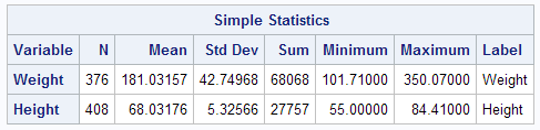
In the sample data, we will use two variables: “Height” and “Weight.” The variable “Height” is a continuous measure of height in inches and exhibits a range of values from 55.00 to 84.41. The variable “Weight” is a continuous measure of weight in pounds and exhibits a range of values from 101.71 to 350.07.

Running the Test

SAS Program

PROC CORR DATA=sample PLOTS=SCATTER(NVAR=all);
   VAR weight height;
RUN;

Output

Tables

The first two tables tell us what variables were analyzed, and their descriptive statistics.

The third table contains the Pearson correlation coefficients and test results.

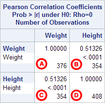
Notice that the correlations in the main diagonal (cells A and D) are all equal to 1. This is because a variable is always perfectly correlated with itself. Notice, however, that the sample sizes are different in cell A (n=376) versus cell D (n=408). This is because of missing data -- there are more missing observations for variable Weight than there are for variable Height, respectively.

The important cells we want to look at are either B or C. (Cells B and C are identical, because they include information about the same pair of variables.) Cells B and D contain the correlation coefficient itself, its p-value, and the number of complete pairwise observations that the calculation was based on.

In cell B (repeated in cell C), we can see that the Pearson correlation coefficient for height and weight is .513, which is significant (p < .001 for a two-tailed test), based on 354 complete observations (i.e., cases with nonmissing values for both height and weight).

Graphs

If you used the PLOTS=SCATTER option in the PROC CORR statement, you will see a scatter plot:

Decision and Conclusions

Based on the results, we can state the following:

• Weight and height have a statistically significant linear relationship (r = 0.51, p < .001).
• The direction of the relationship is positive (i.e., height and weight are positively correlated), meaning that these variables tend to increase together (i.e., greater height is associated with greater weight).
• The magnitude, or strength, of the association is moderate (.3 < | r | < .5).